Introduction

As promised on Thursday, here’s my second pass at a statistical analysis of Canabalt scores. There are some useful results I’ll present right at the start, and then there are some results that are more or less worthless, except that working through my own mistakes helped me to think more clearly about statistical modeling in general and about Poisson models for discrete data in particular.

Rethinking the Problem

First, let’s review the reason why I proposed analyzing the scores in the first place. My goal was to determine whether or not it was reasonable to assume that learned skill really influences your score on Canabalt. If you’ve played for more than ten games in a row, I think it’s intuitively clear that you can warm up and start to do better. Whether or not this holds up to a rigorous analysis is another matter, but I haven’t gotten around to collecting the right data yet.

The mere fact that you can do better with a little bit of practice suggests that the distribution of scores cannot be entirely attributed to chance variation: there’s at least some level of skill that matters. What’s really interesting, though, is how differently different people can perform, regardless of how long they’ve had to warm up.

Originally, I thought that it would be useful to see how well a probabilistic model could explain the distribution of scores. I’ll return to my results fitting probabilistic models in the second part of this post, but I now realize that the basic idea behind this approach was deeply flawed. Even if the distribution of scores looks random, it could easily be the case that it’s the distribution of skill levels that’s random, and that, for any given skill level, your score is more or less deterministic. Though that point doesn’t apply here (where we know that there’s variation in the scores that a single player gets), I think the point in general makes clear that the quality of fit of a probabilistic model to empirical data says nothing about the determinism implicit in the process that generates the data. (Which I should have known already, being a fan of Laplace’s demon.)

Instead, if we want to understand the importance of skill, we should look directly at the difference in average scores between people of seemingly high skill and those of seemingly low skill – that is, we should simply look at the distributions of scores for people with different values of some operationalization of skill level to see how much they differ.

How do we measure skill level? I tried two naïve approaches, and both gave pretty similar results. The first approach is to consider all of the players who have at least one score in the top 10% of scores. The other approach is to consider all of the players whose median score is in the top 10%. I chose the median rather than the mean, because the mean will be biased by a single very high score, which could make these two measures of skill almost identical.

Once you have the two groups defined in your data set using these rules, you can simply perform a t-test to compare the performance of these two groups. Both times, I find that the scores are blatantly different across the two groups. The expert users' mean score is always above 10,000 under both definitions, while the non-expert users' mean score is around 3,500. In short, I’d say that there’s no way that you can realistically argue that skill doesn’t play a part in determining the score you get.

NB: The R code for doing all of this is at the bottom of this post.

Model Fitting

During the original conversation with my fellow graduate students about Canabalt that inspired this post and the one before it, I claimed that the distribution of scores looked like a Poisson distribution based on my (now known to be poor) recollection of the shape of the Poisson distribution. So, when I started my analyses, my first idea was to fit a Poisson distribution to my data using a call to the glm function in R:

glm(scores ~ 1, data = data.set, family = poisson)

To convince myself that this was the correct way to fit a constant Poisson model in R, I derived the maximum likelihood estimator for the mean parameter of a Poisson distribution given a set of sample observations by hand. The math deriving the right parameter estimate is outlined at the bottom of this post and can easily be skipped if that sort of thing is opaque or boring to you.

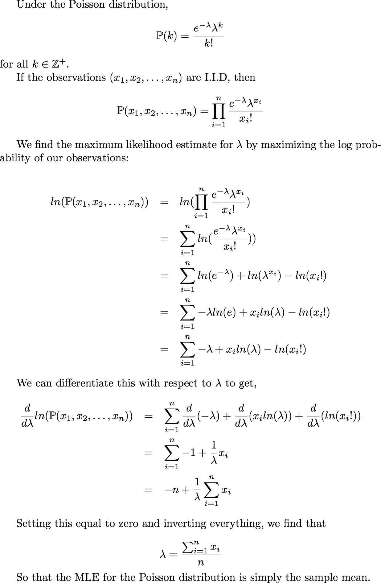
Once you fit this model, you can simulate data from it and see how much it looks like the original data. To refresh your memory, the original score data looks like this:

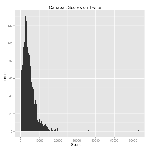
The results of a Poisson simulation look like this:

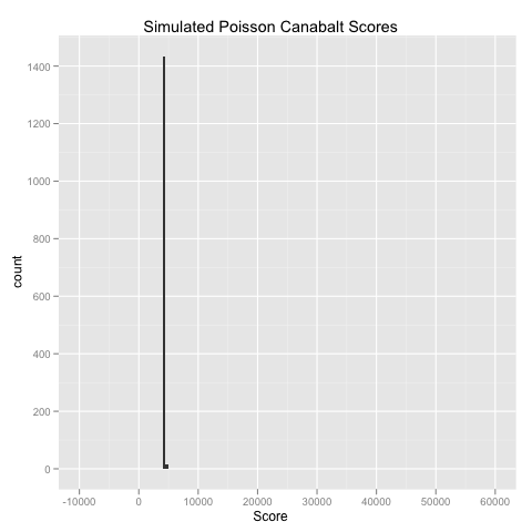
As you can see, this simulation is laughably bad. The Poisson model, lacking a variance parameter, is an absolutely terrible model for the scores from Canabalt. Knowing that I had been basically defeated, I tried a discretized Normal distribution (with a useful independent variance parameter) that was bound to fail because of its symmetry. The results from the Normal distribution look like this:

This is also pretty terrible: there are actually negative results in the data set, no skew at all (which is obviously a given with any parameterization of the Normal distribution) and no outliers. The class of other models I could think of trying beyond these two didn’t seem much more promising, so I didn’t continue on. I hope that’s a reflection of my weak knowledge of probability theory more than anything else.

A Proper Probabilistic Model?

I’d still be interested in seeing whether there is a canonical probability distribution out there that fits the data qualitatively, but I haven’t had any luck searching through lists of distributions online. The desired distribution should:

1. Be integer valued.
2. Be strictly positive.
3. Have heavy tails.

The third point above makes the Poisson distribution, with its small variance, useless, while the second point makes a discretized Normal, with its problematic symmetry, useless. If you have any solutions, please let me know. (I should note that I’ve considered, but decided against, using an over-dispersed Poisson model because I’m not familiar enough with its analytic properties.)

Complete Analysis Code and Results for Across Group Comparisons

You can download my data set here.

data.set <- read.csv('canabalt_data.csv', header = TRUE, sep = ',')

top.ten.score <- as.numeric(quantile(data.set$score, c(0.9)))

top.users <- unique(data.set$user[data.set$score > top.ten.score])

top.users.scores <- with(
    subset(data.set, user %in% top.users),
    score
)
bottom.users.scores <- with(
    subset(data.set, !(user %in% top.users)),
    score
)

t.test(bottom.users.scores, top.users.scores)

#	Welch Two Sample t-test
#
#data:  bottom.users.scores and top.users.scores
#t = -16.7087, df = 196.389, p-value < 2.2e-16
#alternative hypothesis: true difference in means is not equal to 0
#95 percent confidence interval:
# -7743.866 -6108.843
#sample estimates:
#mean of x mean of y
# 3443.313 10369.668

alt.top.users <- c()

for (user in with(data.set, unique(user))) {
    median.user.score <- median(data.set$score[data.set$user == user])
    if (median.user.score > top.ten.score) {
        alt.top.users <- c(alt.top.users, user)
    }
}

alt.top.users.scores <- with(
    subset(data.set, user %in% alt.top.users),
    score
)
alt.bottom.users.scores <- with(
    subset(data.set, !(user %in% alt.top.users)),
    score
)

t.test(alt.bottom.users.scores, alt.top.users.scores)

#	Welch Two Sample t-test
#
#data:  alt.bottom.users.scores and alt.top.users.scores
#t = -16.376, df = 139.206, p-value < 2.2e-16
#alternative hypothesis: true difference in means is not equal to 0
#95 percent confidence interval:
# -9130.290 -7163.108
#sample estimates:
#mean of x mean of y
# 3586.801 11733.500

Derivation of the MLE Analytic Formula for the Poisson Distribution