Using Complex Numbers in R

This post is a continuation of my series dealing with matrix operations for image processing. My next goal is to demonstrate the construction of simple low-pass and high-pass spatial frequency filters in R. It’s easy enough to construct simple versions of these filters in R using the Fast Fourier Transform (also known as the FFT), but, because the FFT is a slightly complicated tool, I’m going to build up to using it progressively over a few posts.

For starters, I want to review the use of complex numbers in R. As always, if you’re interested in reviewing the mathematics of complex numbers, I’d start by browsing references online. The tutorial here seemed good to me at first glance, though I can’t claim to have read it through.

Because complex numbers are implemented in the “base” package, it’s very easy to start working with them. To construct the complex number x + iy, you use complex:

x <- 1
y <- 1

z <- complex(real = x, imaginary = y)

z
# [1] 1+1i

It’s conventional in mathematics to use z to refer to a complex number, so I’ll continue on with that tradition.

As always occurs with mathematical data types in R, you can convert other objects to class “complex” using as.complex:

as.complex(-1)
# [1] -1+0i

And you can test that an object is complex using is.complex:

is.complex(as.complex(-1))
# [1] TRUE

Beyond those standard operations, there are five essential mathematical operations you’d want to use on complex numbers.

First off, you want to be able to extract the real and imaginary components of a complex number. You can do this using Re and Im respectively:

z <- complex(real = 2, imaginary = 1)

Re(z)
# [1] 2

Im(z)
# [1] 1

The (x, y) representation of numbers is easier to understand at first, but a polar coordinates representation is often more practical. You can get the relevant components of this representation by finding the modulus and complex argument of a complex number. In R, you would use Mod and Arg:

z <- complex(real = , imaginary = 1)

Mod(z)
# [1] 1

Arg(z)
# [1] 1.570796

pi / 2
# [1] 1.570796

This corresponds to the intuition that i should be at a distance 1 from the origin and an angle of pi / 2.

Finally, you’ll want to be able to take the complex conjugate of a complex number; to do that in R, you can use Conj:

Conj(z)
# [1] 0-1i

Mod(z) == z * Conj(z)
# [1] TRUE

As you can see, the modulus of z equals z times the conjugate of z, which is exactly what you expect.

Now, historically, complex numbers were invented so that you could find the square root of negative numbers. By default, sqrt does not return a complex number when you ask for the square root of a negative number. Instead, it produces a NaN error, as you can see below:

sqrt(-1)
# [1] NaN
# Warning message:
# In sqrt(-1) : NaNs produced

To get the complex square root, you need to cast your negative number as a complex number using as.complex before applying sqrt:

sqrt(as.complex(-1))

# [1] 0+1i

In practice, complex numbers can be used to solve a huge range of problems, not least of which is the efficient representation of the FFT of an input vector. For fun, I thought I’d show a simple application: building a fractal using the Mandelbrot set.

To quote Wikipedia,

Mathematically the Mandelbrot set can be defined as the set of complex values of c for which the orbit of 0 under iteration of the complex quadratic polynomial z_n+1 = z_n^2 + c remains bounded. That is, a complex number, c, is in the Mandelbrot set if, when starting with z = 0 and applying the iteration repeatedly, the absolute value of z_n never exceeds a certain number (that number depends on c) however large n gets.

We can translate this definition into R pretty easily by making certain assumptions about the exactness we want in our results. For my purposes, I’ll say that a number is in the Mandelbrot set if, after 100 iterations of the Mandelbrot algorithm, it’s never once had a modulus greater than 1,000,000. As you’ll see from the image I produced, this assumption works out pretty well, though it takes some real number crunching to get results out of it for reasonable sized data sets.

in.mandelbrot.set <- function(c, iterations = 100, bound = 1000000) {
    z <- 0

    for (i in 1:iterations) {
        z <- z ** 2 + c
        if (Mod(z) > bound)
        {
            return(FALSE)
        }
    }

    return(TRUE)
}

Once we have this algorithm, we can easily generate an image of the Mandelbrot set by producing a matrix of complex numbers and depicting their inclusion in the set using image:

resolution <- 0.001

sequence <- seq(-1, 1, by = resolution)

m <- matrix(nrow = length(sequence), ncol = length(sequence))

for (x in sequence) {
    for (y in sequence) {
        mandelbrot <- in.mandelbrot.set(complex(real = x, imaginary = y))
        m[round((x + resolution + 1) / resolution), round((y + resolution + 1) / resolution)] <- mandelbrot
    }
}

png('mandelbrot.png')
image(m)
dev.off()

And here’s the resulting image:

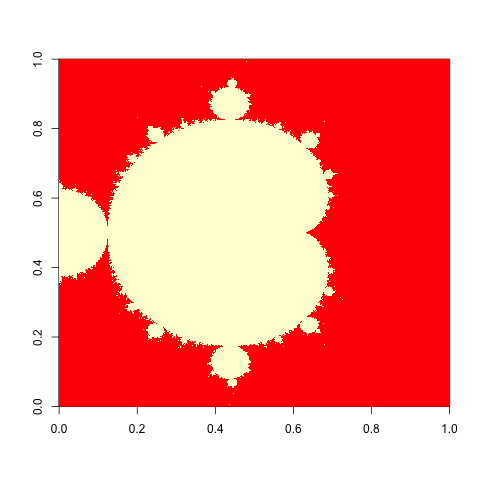
UPDATE: Thanks to Giuseppe for pointing out the rounding error in the original code, producing an image with lines in it.