[UPDATE: As Will points out in the comments, this isn’t really the EM algorithm. There isn’t a proper E step, because there’s no distribution being estimated: there’s only a maximization step that alternates between maximizing the class labels and the slopes. You can think of this algorithm as a degenerate version of EM in the way that naive k-means implements a degenerate form of EM for Gaussian mixtures.]
Last night, Drew Conway showed me a fascinating graph that he made from the R package data we’ve recently collected from CRAN. That graph will be posted and described in the near future, because it has some really interesting implications for the structure of the R package world.
But for the moment I want to talk about the use of mixture modeling when you have a complex regression problem. I think it’s easiest to see some example data to motivate my interest in this topic, so here we go:
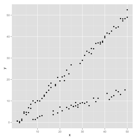
If you’ve never seen data like this, let’s just make sure it’s clear how you could have ended up with a plot that looks this way. We could end up with data like this if we had two classes of data points that each separately obey a standard linear regression model, but the models have different slopes for points from each of the two classes of data. In other words, this is the sort of data set you might fit using a varying-slope regression model – if you knew about the classes coming in to the problem. To make this idea really clear, here’s the simulation code that generated the plot I’ve just shown you.
N <- 100

true.classes <- sample(c(0, 1), N, replace = TRUE)

x <- rep(1:50, 2)

y <- rep(NA, N)

beta <- c(0.3, 1.0)

for (i in 1:N) {
    y[i] <- beta[true.classes[i] + 1] * x[i] + rnorm(1)
}

png('unlabeled.png')
qplot(x, y, geom = 'point')
dev.off()
But what do you do when you don’t know anything about the classes because you’ve only discovered them after visualizing your data? It should be obvious that no amount of regression trickery is going to give us the class information we’re missing. And we also can’t fit a varying slope regression without some sort of class information. It would seem that we can’t get started at all given standard regression techniques, because we have a chicken-and-egg problem where we need either the class labels or the regression parameters to infer the other missing piece of the puzzle.
The solution to this problem may amaze readers who don’t already know the EM algorithm and degenerate forms of EM, because it’s so shockingly simple and seemingly cavalier in its approach: we make up for the missing data by just making new data up out of thin air.
Seriously. The approach I’ll describe reliably works and it works for two reasons that are obvious in retrospect once someone’s told them to you:
- If we have an algorithm that will eventually reach the best solution to a problem from any starting point, then we can make up for missing data by randomly selecting values for what we’re missing and moving on from there. We don’t have to be paralyzed by the seemingly insurmountable problem of doubly missing data, because using arbitrary data is enough for us to get started. Now if that’s not data hacking, I don’t know what is.
- The first claim isn’t just hypothetical when there’s a finite number of possible classes each point could belong to: our algorithm really will eventually reach the best solution, because each step of the algorithm will always give us a better solution than before, and there are only finitely many steps the algorithm can take, because there is only a finite number of possible class label assignments it could use.
With that said, let’s go through the details for this problem with example code.
First, we have to make up imaginary class labels.
inferred.classes <- sample(c(0, 1), N, replace = TRUE)
Then we’ll plot this assignment of classes to see how well it matches the structure we see visually:
png(paste('state_', 0, '.png', sep = ''))
qplot(x, y, geom = 'point', color = inferred.classes)
dev.off()
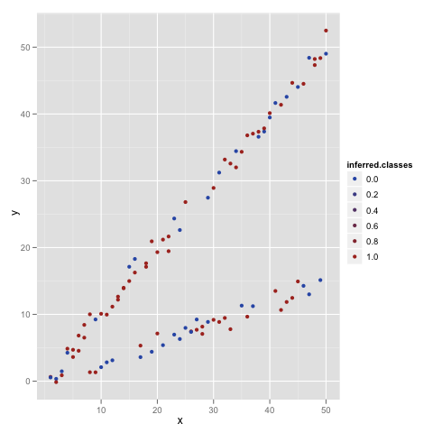
This assignment doesn’t look good at all. That’s not surprisingly given that we made it up without any reference to the rest of our data. But it’s actually quite easy to go from this made up set of labels to a better set. How? By fitting a varying-slope regression, calculating the errors at each data point for both possible class labels, and then re-assigning data points to the class that makes the errors smallest. We can do that with the following very simple code:
my.data <- data.frame(Y = y, X = x, Class = inferred.classes)

lm.fit <- lm(Y ~ X + X:Class - 1, data = my.data)

for (i in 1:N) {
    error.zero <- (
        y[i] - predict(lm.fit, data.frame(Y = y[i], X = x[i], Class = ))
    )^2
    error.one <- (
        y[i] - predict(lm.fit, data.frame(Y = y[i], X = x[i], Class = 1))
    )^2

    if (error.zero < error.one) {
        inferred.classes[i] <- 0
    } else {
        inferred.classes[i] <- 1
    }
}
Here we fit a linear regression with two slopes, depending on the class being 0 or 1, and we’ve thrown out any intercept for simplicity. Then we determine which of the two classes would make the data more likely given the slopes we inferred using our imaginary classes. This actually makes a huge improvement in just one step:
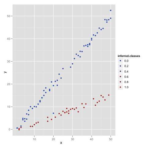
Luckily for us, there’s only data point that’s not been assigned properly, so we can just loop over the steps we took one more time to clean up our model to near perfection:
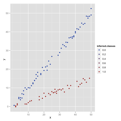
And that’s it.
[EDIT: Fixed a typo in the example code that actually made the algorithm work faster, but only because it coincided with the structure of the problem.]