Bayesian Nonparametrics in R

On July 25th, I’ll be presenting at the Seattle R Meetup about implementing Bayesian nonparametrics in R. If you’re not sure what Bayesian nonparametric methods are, they’re a family of methods that allow you to fit traditional statistical models, such as mixture models or latent factor models, without having to fully specify the number of clusters or latent factors in advance.

Instead of predetermining the number of clusters or latent factors to prevent a statistical algorithm from using as many clusters as there are data points in a data set, Bayesian nonparametric methods prevent overfitting by using a family of flexible priors, including the Dirichlet Process, the Chinese Restaurant Process or the Indian Buffet Process, that allow for a potentially infinite number of clusters, but nevertheless favor using a small numbers of clusters unless the data demands using more.

This flexibility has several virtues:

1. You don’t have to decide how many clusters are present in your data before seeing the results of your analysis. You just specify the strength of a penalty for creating more clusters.
2. The results of a fitted Bayesian nonparametric model can be used as informed priors when you start processing new data. This is particularly important if you are writing an online algorithm: the use of a prior like the Chinese Restaurant Process that, in principle, allows the addition of new clusters at any time means that you can take advantage of all the information you have about existing clusters without arbitrarily forcing new data into those clusters: if a new data point is unique enough, it will create its own cluster.

To give you a sense of how Bayesian nonparametric methods work, I recently coded up the newly published dp-Means algorithm, which provides a deterministic implementation of a k-means like algorithm that allows for a potentially infinite number of clusters, but, in practice, only uses a small number of clusters by penalizing the creation of additional clusters. This penalty comes from a parameter, lambda, that the user specifies before fitting the model.

The series of images below shows how the dp-Means algorithm behaves when you turn it loose on a data set with four distinct Gaussian clusters. Each image represents a higher penalty for using more clusters.

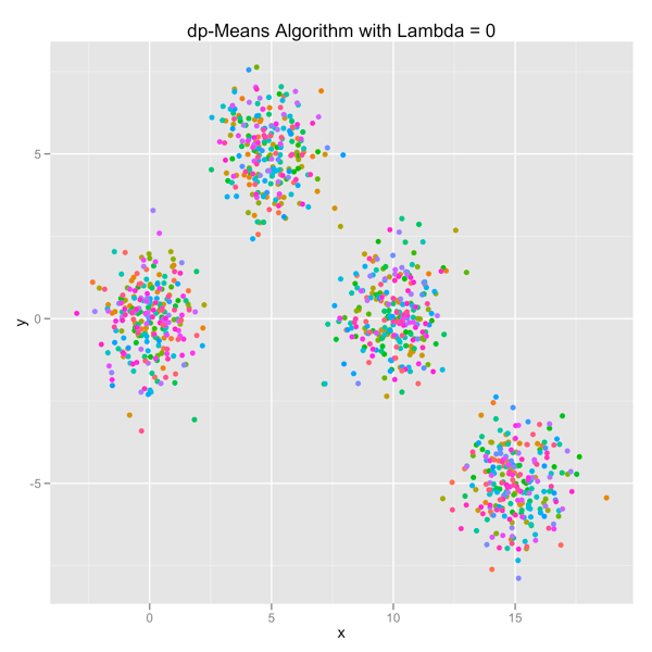
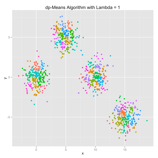
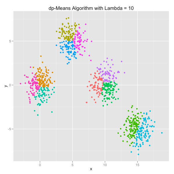
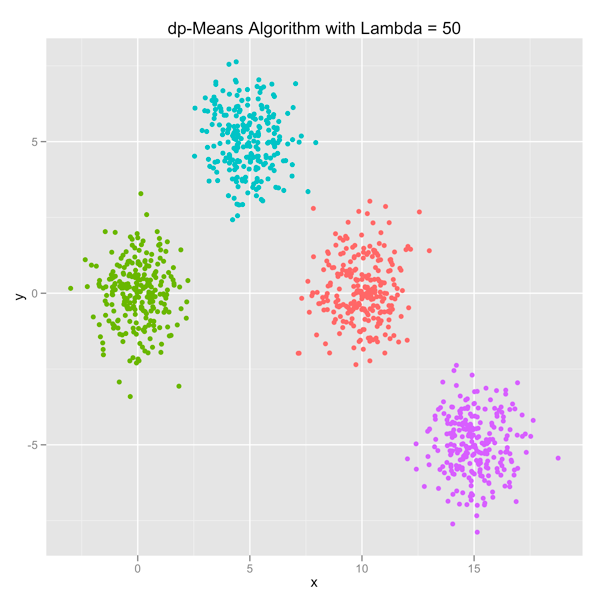
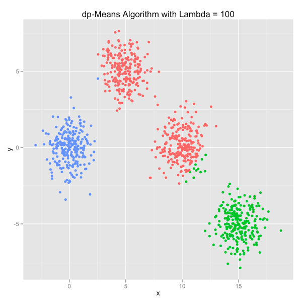
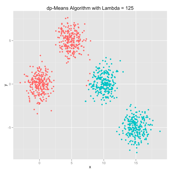
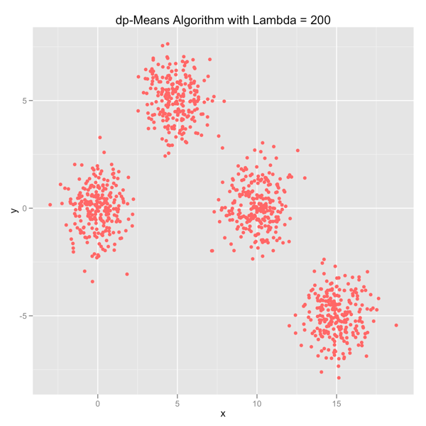
As you can see, you can shift the model from a preference for using many clusters to using only one by manipulating the lambda parameter. If you’re interested in learning more and will be in the Seattle area in late July, come out.