Introduction

Statistically-trained readers of this blog will be very familiar with the Central Limit Theorem, which describes the asymptotic sampling distribution of the mean of a random vector composed of IID variables. Some of the most interesting recent work in mathematics has been focused on the development of increasingly powerful proofs of a similar law, called the Circular Law, which describes the asymptotic sampling distribution of the eigenvalues of a random matrix composed of IID variables.

Julia, which is funded by one of the world’s great experts on random matrix theory, is perfectly designed for generating random matrices to experiment with the Circular Law. The rest of this post shows how you might write the most naive sort of Monte Carlo study of random matrices in order to convince yourself that the Circular Law really is true.

Details

In order to show off the Circular Law, we need to be a bit more formal. We’ll define a random matrix \(M\) as an \(N\)x\(N\) matrix composed of \(N^{2}\) IID complex random variables, each with mean \(0\) and variance \(\frac{1}{N}\). Then the distribution of the \(N\) eigenvalues asymptotically converges to the uniform distribution over the unit disc. I think it’s easiest to see this by doing a Monte Carlo simulation of the eigenvalues of random matrices composed of Gaussian variables for five values of \(N\):

f = open("eig.tsv", "w")

println(f, join(["N", "I", "J", "Re", "Im"], "\t"))

ns = [1, 2, 5, 25, 50]
sims = 100

for n in ns
    for i in 1:sims
        m = (1 / sqrt(n)) * randn(n, n)
        e, v = eig(m)
        for j in 1:n
            println(f, join([n, i, j, real(e[j]), imag(e[j])], "\t"))
        end
    end
end

close(f)

The results from this simulation are shown below:

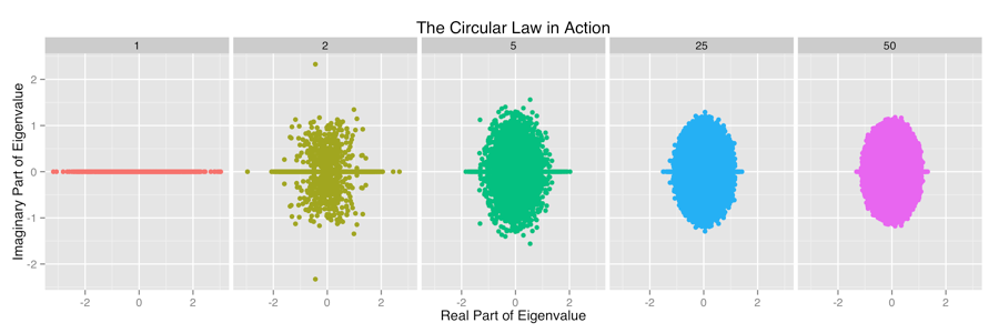
These images highlight two important patterns:

1. For the entry-level Gaussian distribution, the distribution of eigenvalues converges on the unit circle surprisingly quickly.
2. There is a very noticeable excess of values along the real line that goes away much more slowly than the movement towards the unit disk.

If you’re interested in exploring this topic, I’d encourage you to try two things:

1. Obtain samples from a larger variety of values of \(N\).
2. Construct samples from other entry-level distributions than the Gaussian distribution used here.

PS: Drew Conway wants me to note that Julia likes big matrices.