Introduction / Warning

Any traditional introductory statistics course will teach students the definitions of modes, medians and means. But, because introductory courses can’t assume that students have much mathematical maturity, the close relationship between these three summary statistics can’t be made clear. This post tries to remedy that situation by making it clear that all three concepts arise as specific parameterizations of a more general problem.

To do so, I’ll need to introduce one non-standard definition that may trouble some readers. In order to simplify my exposition, let’s all agree to assume that \(0^0 = 0\). In particular, we’ll want to assume that \(\lvert 0 \rvert^0 = 0\), even though \(\lvert \epsilon \rvert^0 = 1\) for all \(\epsilon > 0\). This definition is non-standard, but it greatly simplifies what follows and emphasizes the conceptual unity of modes, medians and means.

Constructing a Summary Statistic

To see how modes, medians and means arise, let’s assume that we have a list of numbers, \((x_1, x_2, \ldots, x_n)\), that we want to summarize. We want our summary to be a single number, which we’ll call \(s\). How should we select \(s\) so that it summarizes the numbers, \((x_1, x_2, \ldots, x_n)\), effectively?

To answer that, we’ll assume that \(s\) is an effective summary of the entire list if the typical discrepancy between \(s\) and each of the \(x_i\) is small. With that assumption in place, we only need to do two things: (1) define the notion of discrepancy between two numbers, \(x_i\) and \(s\); and (2) define the notion of a typical discrepancy. Because each number \(x_i\) produces its own discrepancy, we’ll need to introduce a method for aggregating the individual discrepancies to order to say something about the typical discrepancy.

Defining a Discrepancy

We could define the discrepancy between a number \(x_i\) and another number \(s\) in many ways. For now, we’ll consider only three possibilities. All of these three options satisfies a basic intuition we have about the notion of discrepancy: we expect that the discrepancy between \(x_i\) and \(s\) should be \(0\) if \(\lvert x_i - s \rvert = 0\) and that the discrepancy should be greater than \(0\) if \(\lvert x_i - s \rvert > 0\). That leaves us with one obvious question: how much greater should the discrepancy be when \(\lvert x_i - s \rvert > 0\)?

To answer that question, let’s consider three definitions of the discrepancy, \(d_i\):

1. \(d_i = \lvert x_i - s \rvert^0\)
2. \(d_i = \lvert x_i - s \rvert^1\)
3. \(d_i = \lvert x_i - s \rvert^2\)

How should we think about these three possible definitions?

The first definition, \(d_i = \lvert x_i - s \rvert^0\), says that the discrepancy is \(1\) if \(x_i \neq s\) and is \(0\) only when \(x_i = s\). This notion of discrepancy is typically called zero-one loss in machine learning. Note that this definition implies that anything other than exact equality produces a constant measure of discrepancy. Summarizing \(x_i = 2\) with \(s = 0\) is no better nor worse than using \(s = 1\). In other words, the discrepancy does not increase at all as \(s\) gets further and further from \(x_i\). You can see this reflected in the far-left column of the image below:

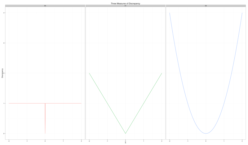
The second definition, \(d_i = \lvert x_i - s \rvert^1\), says that the discrepancy is equal to the distance between \(x_i\) and \(s\). This is often called an absolute deviation in machine learning. Note that this definition implies that the discrepancy should increase linearly as \(s\) gets further and further from \(x_i\). This is reflected in the center column of the image above.

The third definition, \(d_i = \lvert x_i - s \rvert^2\), says that the discrepancy is the squared distance between \(x_i\) and \(s\). This is often called a squared error in machine learning. Note that this definition implies that the discrepancy should increase super-linearly as \(s\) gets further and further from \(x_i\). For example, if \(x_i = 1\) and \(s = 0\), then the discrepancy is \(1\). But if \(x_i = 2\) and \(s = 0\), then the discrepancy is \(4\). This is reflected in the far right column of the image above.

When we consider a list with a single element, \((x_1)\), these definitions all suggest that we should choose the same number: namely, \(s = x_1\).

Aggregating Discrepancies

Although these definitions do not differ for a list with a single element, they suggest using very different summaries of a list with more than one number in it. To see why, let’s first assume that we’ll aggregate the discrepancy between \(x_i\) and \(s\) for each of the \(x_i\) into a single summary of the quality of a proposed value of \(s\). To perform this aggregation, we’ll sum up the discrepancies over each of the \(x_i\) and call the result \(E\).

In that case, our three definitions give three interestingly different possible definitions of the typical discrepancy, which we’ll call \(E\) for error:

$$ E_0 = \sum_{i} \lvert x_i - s \rvert^0. $$

$$ E_1 = \sum_{i} \lvert x_i - s \rvert^1. $$

$$ E_2 = \sum_{i} \lvert x_i - s \rvert ^2. $$

When we write down these expressions in isolation, they don’t look very different. But if we select \(s\) to minimize each of these three types of errors, we get very different numbers. And, surprisingly, each of these three numbers will be very familiar to us.

Minimizing Aggregate Discrepancies

For example, suppose that we try to find \(s_0\) that minimizes the zero-one loss definition of the error of a single number summary. In that case, we require that

$$ s_0 = \arg \min_{s} \sum_{i} \lvert x_i - s \rvert^0. $$

What value should \(s_0\) take on? If you give this some extended thought, you’ll discover two things: (1) there is not necessarily a single best value of \(s_0\), but potentially many different values; and (2) each of these best values is one of the modes of the \(x_i\).

In other words, the best single number summary of a set of numbers, when you use exact equality as your metric of error, is one of the modes of that set of numbers.

What happens if we consider some of the other definitions? Let’s start by considering \(s_1\):

$$ s_1 = \arg \min_{s} \sum_{i} \lvert x_i - s \rvert^1. $$

Unlike \(s_0\), \(s_1\) is a unique number: it is the median of the \(x_i\). That is, the best summary of a set of numbers, when you use absolute differences as your metric of error, is the median of that set of numbers.

Since we’ve just found that the mode and the median appear naturally, we might wonder if other familiar basic statistics will appear. Luckily, they will. If we look for,

$$ s_2 = \arg \min_{s} \sum_{i} \lvert x_i - s \rvert^2, $$

we’ll find that, like \(s_1\), \(s_2\) is again a unique number. Moreover, \(s_2\) is the mean of the \(x_i\). That is, the best summary of a set of numbers, when you use squared differences as your metric of error, is the mean of that set of numbers.

To sum up, we’ve just seen that the three most famous single number summaries of a data set are very closely related: they all minimize the average discrepancy between \(s\) and the numbers being summarized. They only differ in the type of discrepancy being considered:

1. The mode minimizes the number of times that one of the numbers in our summarized list is not equal to the summary that we use.
2. The median minimizes the average distance between each number and our summary.
3. The mean minimizes the average squared distance between each number and our summary.

In equations,

1. \(\text{The mode of } x_i = \arg \min_{s} \sum_{i} \lvert x_i - s \rvert ^0\)
2. \(\text{The median of } x_i = \arg \min_{s} \sum_{i} \lvert x_i - s \rvert ^1\)
3. \(\text{The mean of } x_i = \arg \min_{s} \sum_{i} \lvert x_i - s \rvert ^2\)

Summary

We’ve just seen that the mode, median and mean all arise from a simple parametric process in which we try to minimize the average discrepancy between a single number \(s\) and a list of numbers, \(x_1, x_2, \ldots, x_n\) that we try to summarize using \(s\). In a future blog post, I’ll describe how the ideas we’ve just introduced relate to the concept of \(L_p\) norms. Thinking about minimizing \(L_p\) norms is a generalization of taking modes, medians and means that leads to almost every important linear method in statistics – ranging from linear regression to the SVD.

Thanks

Thanks to Sean Taylor for reading a draft of this post and commenting on it.