Over the last few months, I’ve had a lot of conversations with people about the use of winsorization to deal with heavy-tailed data that is positively skewed because of large outliers. After a conversation with my friend Chris Said this past week, it became clear to me that I needed to do some simulation studies to understand the design space of techniques for dealing with outliers.

In this post, I’m going to write up my current understanding of the topic. To motivate my perspective, I’m going to describe a specific inferential problem. Trying to solve that problem will require me to explore a small portion of the design space of algorithms for dealing with outliers. It is not at all clear to me how well the conclusions I reach will generalize to other settings, but my hope is that a thorough examination of one specific problem will touch on some of the core issues that would arise in other settings. I’ve also put the code for this simulation study on GitHub so that others can easily build variants of it.

Defining Outliers

To simplify things, I’m going to define an outlier as any value greater than a certain percentile of all of the observed data points. For example, I might say that all observations above the 90th percentile are outliers. In this case, I will say that the “outlier window” is 10%, because I will consider all observations above the (100 - 10)th percentile to be outliers. This outlier window parameter is the first dimension of the design space that I want to understand. Most applications employ a very gentle outlier window, which labels no more than 5% of observations as outliers. But sometimes one sees more radical windows used. In this post, I will consider windows ranging from 1% up to 40%.

Outlier Removal

Given that we’ve flagged some observations as outliers, what do we do with them? I’ll consider three options:

• Do nothing and leave the data unadjusted.
• Discard all of the outliers. The removal of extreme values is usually called trimming or truncation.
• Replace all of the outliers with the largest value that is not considered an outlier. The replacement of extreme values is usually called winsorization.

The Data Generation Process and Inferential Problem

As a further simplification, I’m only going to consider a single inferential problem: estimating the difference in means between two groups of observations. In this problem, I will generate data as follows:

• Draw \(n\) IID observations from a distribution \(D\). Label this set of observations as Group A.
• Draw \(n\) additional IID observations from the same distribution \(D\) and add a constant, \(\delta\), to every one of them. Label this set of observations as Group B.

In this post, the distribution, \(D\), that I will use is a log-normal distribution with mean 1.649 and standard deviation 2.161. These strange values correspond to a mean of 0 and a standard deviation of 1 on the pre-exponentiation scale used by my RNG.

Given that distribution, \(D\), I’ll consider three values of \(\delta\): 0.00, 0.05 and 0.10. Each value of \(\delta\) defines a new distribution, \(D^{\prime}\).

To contrast these distributions, I want to consider the quantity: \(\delta = \mathbb{E}[D^{\prime}] - \mathbb{E}[D]\). The outlier approaches I’ll consider will lead to several different estimators. I’ll refer to each of these estimators as \(\hat{\delta}\). From each estimator, I’ll construct point estimates and interval estimates; I’ll also conduct hypothesis tests based on the estimators using t-tests.

Selection of Outlier Windows

Given that we have two data sets, \(A\) and \(B\), applying outlier detection requires us to make another decision about our position in design space: which data sets do we use to compute the percentile that defines the outlier threshold?

I’ll consider three options:

• Compute a single percentile from a new data set formed by combining A and B. In the results, I’ll call this the “shared threshold” rule.
• Compute a single percentile using data from A only. In the results, I’ll call this the “threshold from A” rule.
• Compute two percentiles: one using data from A only and another using data from B only. We will then apply the threshold from A to A’s data and apply the threshold from B to B’s data. In the results, I’ll call this the “separate thresholds” rule.

Combining this new design decision with the others already mentioned, the design space I’m interested in has three dimensions:

• The outlier window.
• The method for addressing outliers, which is either (a) no adjustment, (b) trimming, or (c) winsorization.
• The data set used to compute the outlier threshold, which is a shared threshold, a separate threshold or a threshold derived from A’s observations only.

Results

I consider the quality of inferences in terms of several metrics:

• Point Estimation:
  • The bias of \(\hat{\delta}\) as an estimator of \(\delta\).
  • The RMSE of \(\hat{\delta}\) as an estimator of \(\delta\).
• Interval Estimation:
  • The coverage probability of nominal 95% CI’s for \(\delta\) built around \(\hat{\delta}\).
• Hypothesis Testing:
  • The false positive rate of a t-test when \(\delta = 0.00\).
  • The false negative rates of t-tests when \(\delta = 0.05\) or \(\delta = 0.10\).

Point Estimation

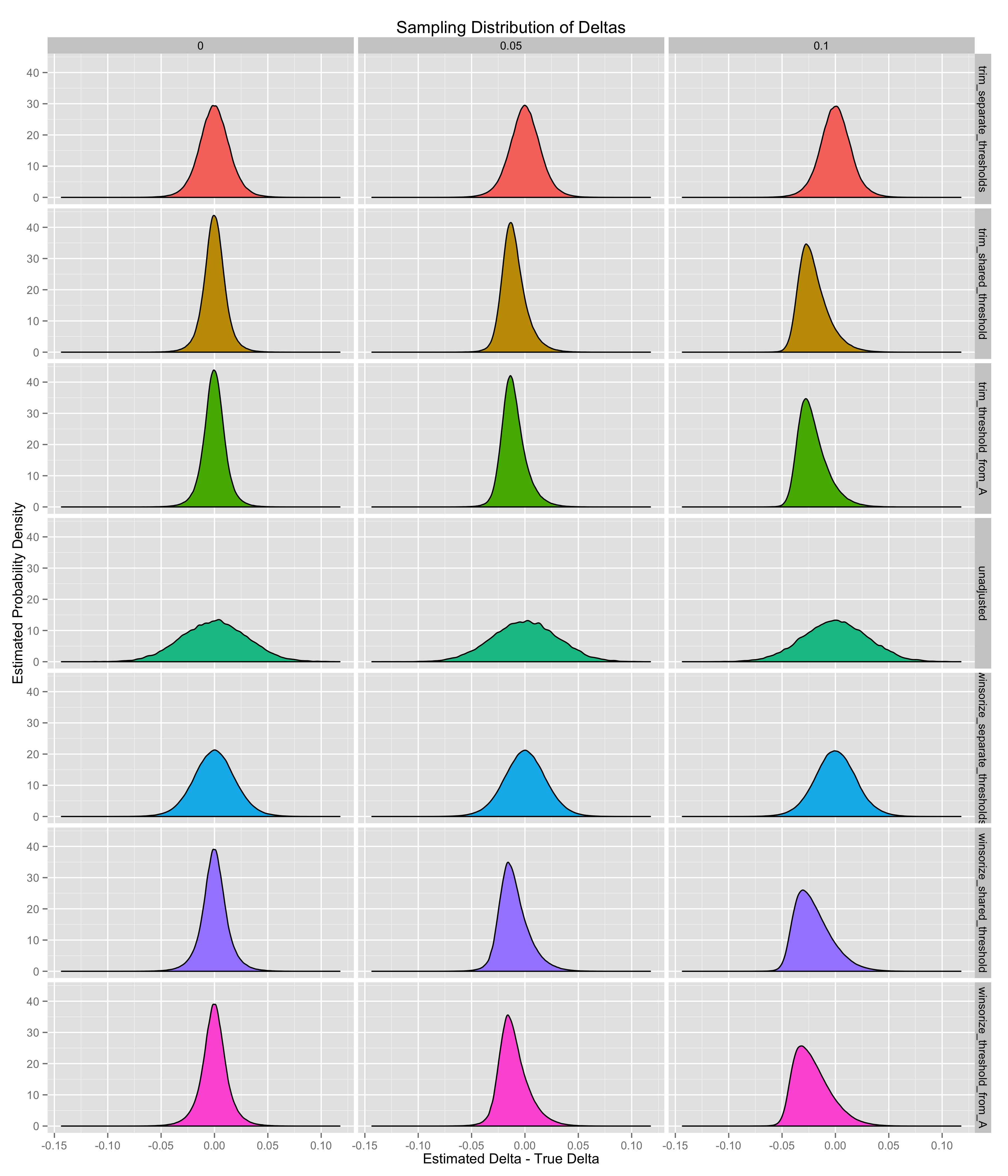
The results for the point estimation problem are shown graphically below. I begin by plotting KDE’s of the sampling distributions of the seven estimators I’m considering, which give an intuition for all of the core results shown later. The columns in these plots reflect the different values of \(\delta\), which are either 0.00, 0.05 or 0.10.

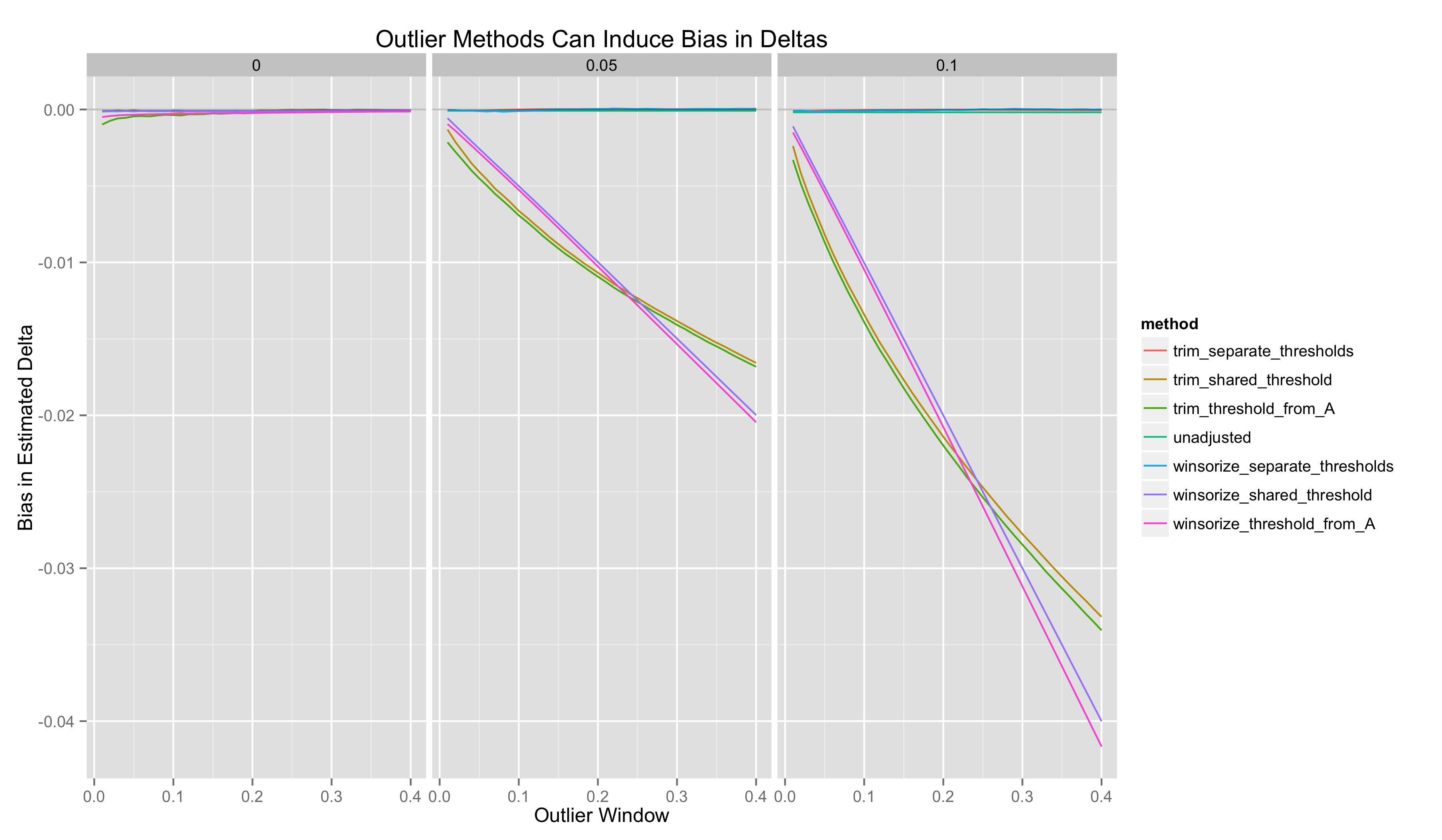
Next I plot the bias of these estimators as a function of the outlier window. I split these plots according to the true value of \(\delta\):

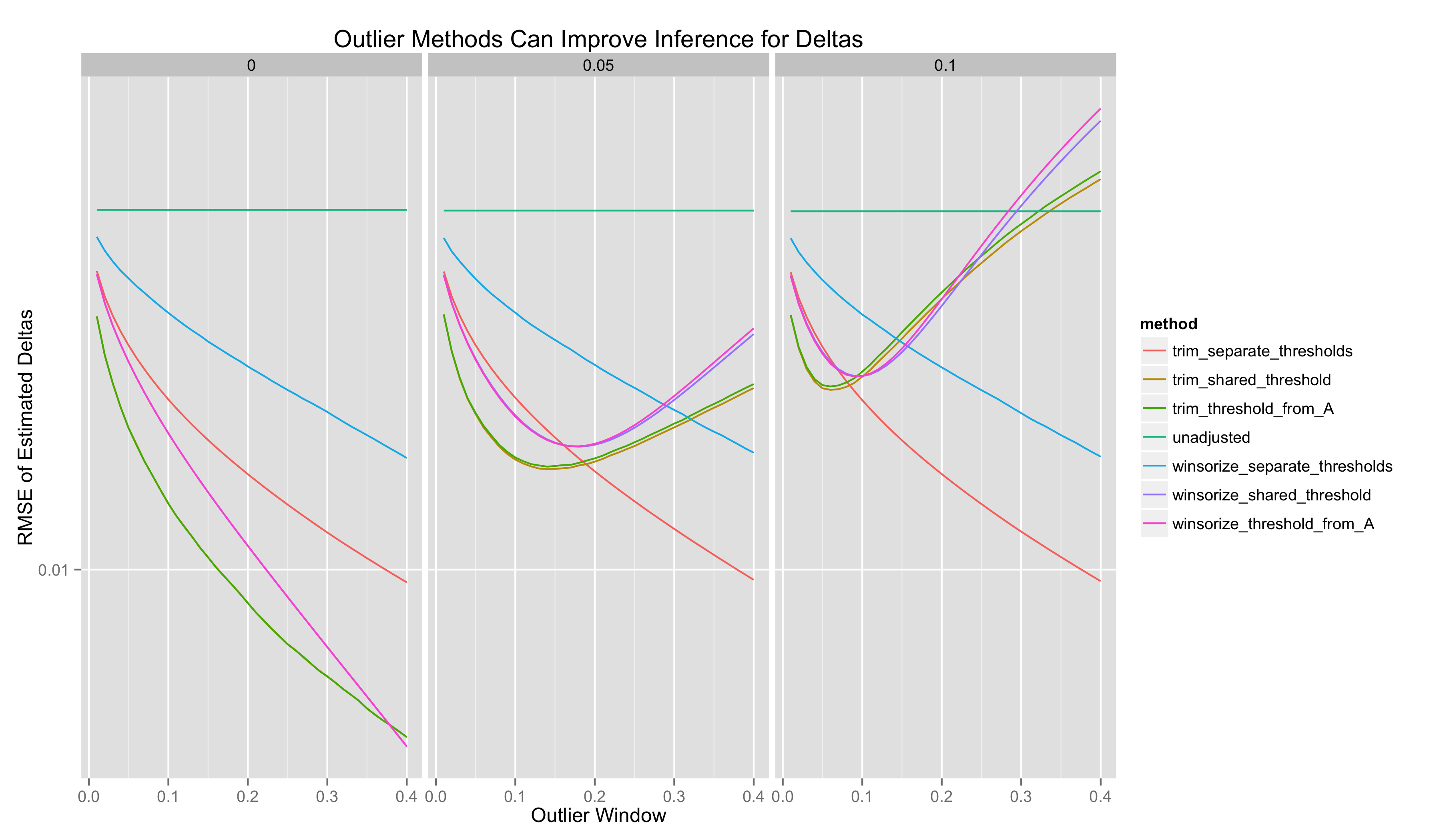
Finally, I plot the RMSE of these estimators as a function of the outlier window, again splitting the plots according to the true value of \(\delta\):

Interval Estimation

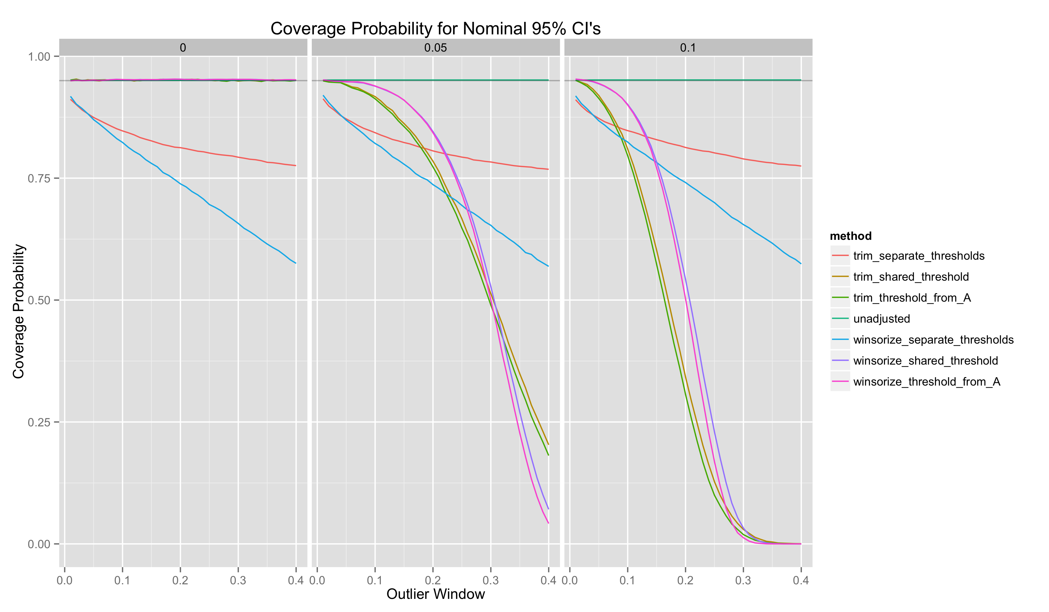
To assess the quality of interval estimates derived from these estimators of \(\hat{\delta}\), I plot the empirical coverage probability of nominal 95% CI’s:

Hypothesis Testing

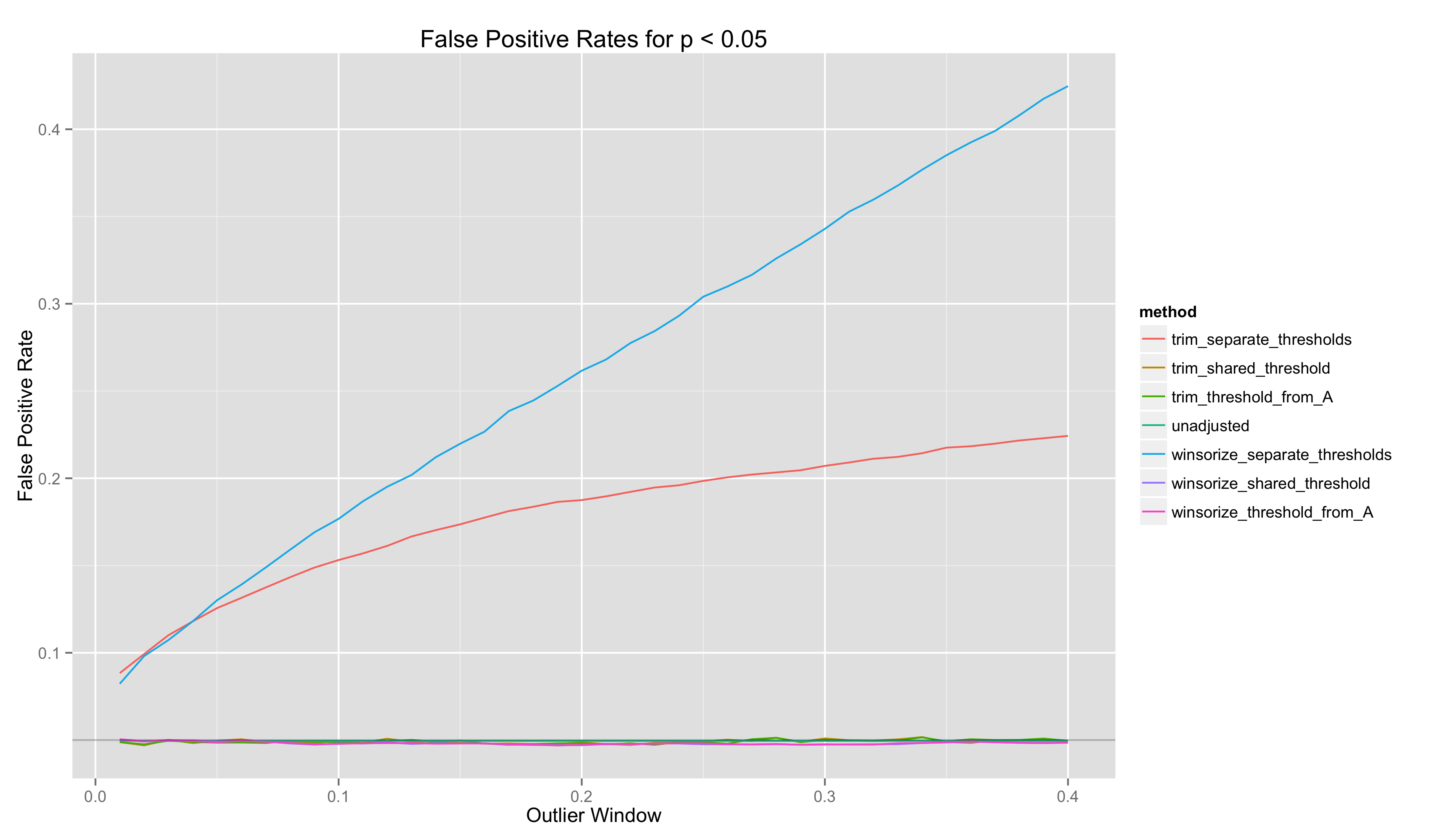
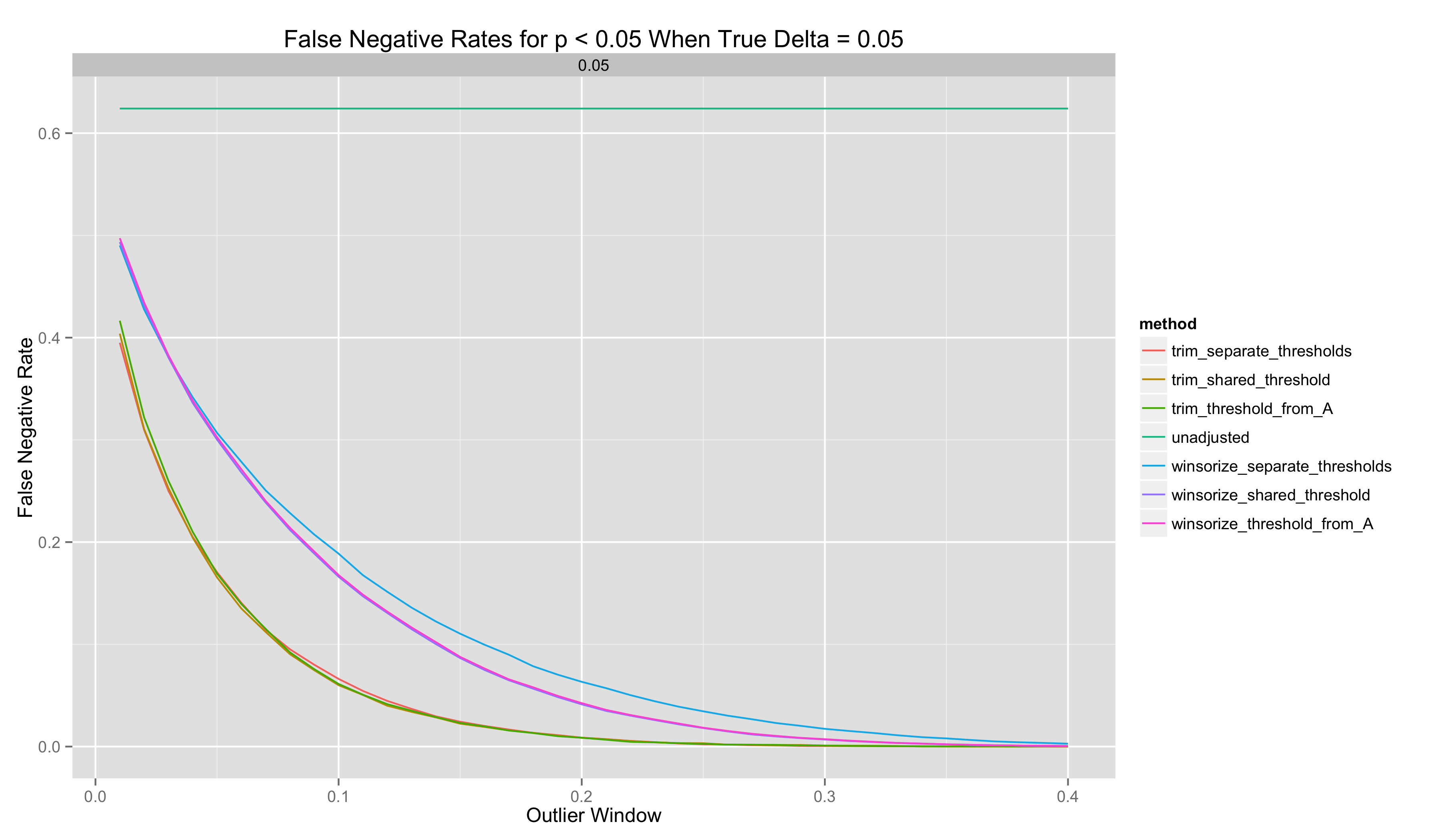
In this last set of analyses, I plot the false positive and false negative rates as a function of the outlier window:

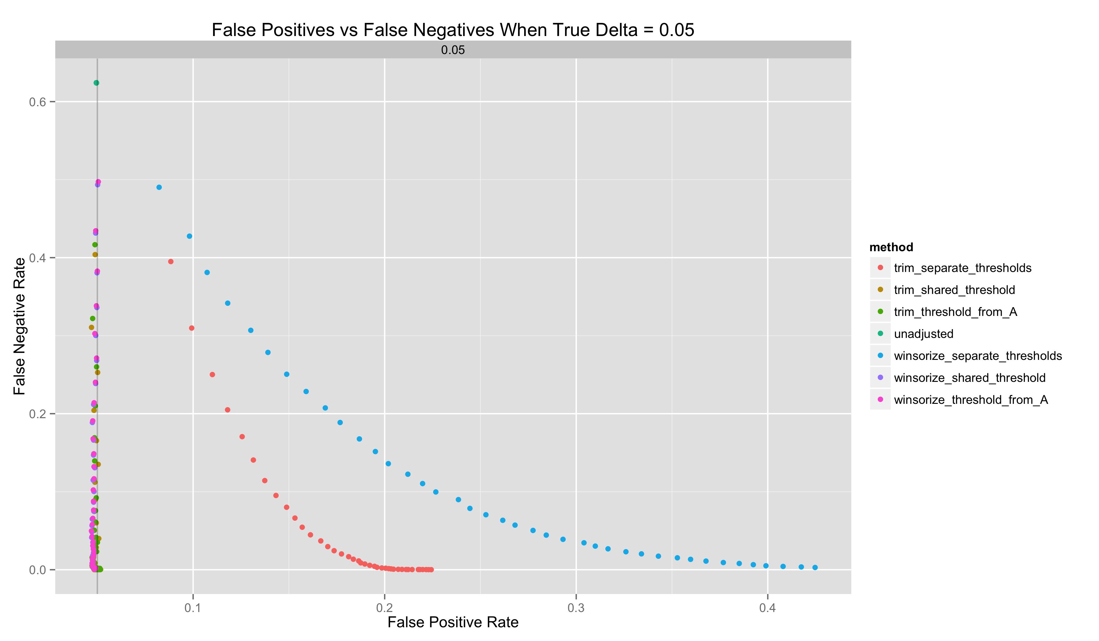
And, for one final analysis, I include a plot of false positive rate when \(\delta = 0.00\) vs false negative rate when \(\delta = 0.05\). This makes it easier to see which methods are strictly dominated by others:

Take-Aways

• Both winsorization and trimming can improve the quality of point estimates of \(\delta\). But they can make inferences worse because they can introduce bias into these point estimates. The only way to prevent bias is to compute outlier thresholds in Groups A and B separately.
• There is sometimes an optimal outlier window that minimizes the RMSE of point estimates of \(\delta\). It is not clear how to calculate this without knowing the ground truth parameter that you are trying to infer. Perhaps cross-validation would work. Importantly, choosing a bad value for the outlier window makes both winsorization and trimming inferior to doing no adjustment.
• Both winsorization and trimming can improve the FP/FN tradeoffs made in a system, although one must use outlier thresholds that are shared across the A and B groups to reap these benefits
• CI’s only provide the desired coverage probabilities when the outlier window is very small.

Putting all this together, my understanding is that there is no universally best method without a more complex approach to outlier control. Whether winsorization or trimming improves the quality of inference depends on the structure of the data being analyzed and the inferential approach being used. Some methods work well for point estimation and interval estimation, others work well for hypothesis testing. No method universally beats out the option of doing no adjustment for outliers.

A Note about Likely Failures of Generalization

If you consider a different kind of difference between the A and B sets of observations than the constant additive difference rule that I’ve considered, I am fairly sure that the conclusions I’ve reached will not apply.